Data Release 1 is Now Avilable!
NASA ADS Page: Coming Soon
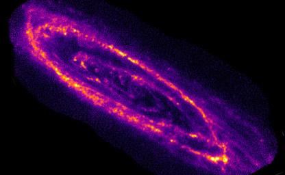
This paper detailed (in possibly too much detail!) how we made our SCUBA-2 images. Ground-based sub-mm images of faint large-angular size objects has been a challenge in the past, mainly due to the fluctuating atmosphere. In this paper we outline how we tune the pipeline to optimise the structures we recover, how we used space-based data to recover the largest-angular scales, and measure the fidelity of our final image. We also predict the contamination of our 850µm due to the CO(J=3-2) line. Our first images are shown in the image below. Some more details on each aspect of the paper is given below.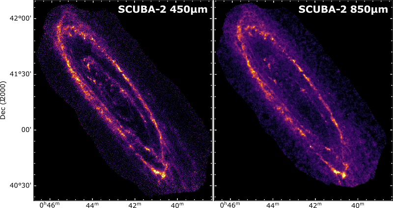
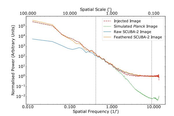
An illustration of how our feathering restores large-scale emission. The red line is the 'true' angular
power spectra of the source. The blue line is the power spectra of just the SCUBA-2 data, when the orange line shows the power spectra after the
feathering is completed (this is much closer to the 'true' red line).
Faint large-angular sized objects (such as nearby galaxies) have always been a challenge from the ground, as variations in the atmosphere can dominate over your emission
requiring harsh filtering to be applied. To overcome this limitation we make combine our data with lower resolution space based data, in this case Planck at 850µm and
Herschel at 450µm, using a process called feathering.
Conceptually the feathering is reasonably simple, with a few simple steps (of course the tricky bits are in the detail):
The SCUBA-2 pipeline has many, many, parameters that can be tweeked to try and optimise the data reduction. What is probably most unique with our analysis is we investigate how the inclusion of principal component analysis can be used so that the high-pass filtering can be relaxed. We also investigate a range of parameters including the 'mask' used, the map-tolerance, and feathering filter settings. This optimisation is actually more challenging at 850µm than 450µm, as the resolution of Planck is significantly lower than that of Herschel.
Another problem we had to overcome is the shear amount of data we had to reduce in one go, unlike deep cosmology surveys we can't reduce an observation individually (as we need to identify the faint structures). So we could reduce the data in a reasonable time we wrote a new version of 'skyloop' called 'scubaDuperSkyloop', this is more parallel version with multiple versions of makemap being able to run on a machine simultaneously, as well as on multiple machines. This script is available on our software page.
 The CO(J=3-2) line for redshift zero sources lies within the 850µm bandpass and in some nearby galaxies can be a large contaminant (up to 30%). We perform a two step
process to predict the CO(J=3-2) line flux; first we use our HARP observations to train a model where we use a variety of maps including WISE, Herschel Dust parameters, SFR, and
most importantly the CARMA(J=1-0) data (as shown in the Figure). The second stage is we use our model with CARMA observations as well as HARP regions not used in stage one as our
truth data (this stage is useful as the CARMA covers a much larger area than our HARP data), to train our model for the datasets that cover the entire galaxy.
The CO(J=3-2) line for redshift zero sources lies within the 850µm bandpass and in some nearby galaxies can be a large contaminant (up to 30%). We perform a two step
process to predict the CO(J=3-2) line flux; first we use our HARP observations to train a model where we use a variety of maps including WISE, Herschel Dust parameters, SFR, and
most importantly the CARMA(J=1-0) data (as shown in the Figure). The second stage is we use our model with CARMA observations as well as HARP regions not used in stage one as our
truth data (this stage is useful as the CARMA covers a much larger area than our HARP data), to train our model for the datasets that cover the entire galaxy.
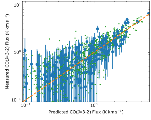
Caption: The measured CO(J=3-2) from our HARP data versus our prediction using various images including the CARMA CO(J=1-0) data.
The green data points are our training set (80% of pixels), and the blue our 'test' set (20% of pixels). The orange line is the 1:1 (or perfect) relation.
In the paper we analyse the fidelity of our final maps, creating bespoke uncertainty maps, and calibrate our images. We typically reach a sensitivity ~2.0 and ~3 mJy beam-1 at 850 and 450µm, respectively, in the 10 kpc ring, with a peak sensitivity in the central regions of 1.5 and 20.6 mJy beam-1 at 850 and 450 µm, respectively. Full details of the maps can be found on our Data Release page
Data Release 1 is Now Avilable!
If you from one of the EAO partners and want to get involved, go to the team page, and find your local contact. If you have any other questions about HASHTAG you can use the contact details below, or if you hvae a specific question about a paper contact the lead author.
The JCMT is operated by the East Asian Observatory association. For more information about the JCMT and EAO click on the icon below.