Data Release 1

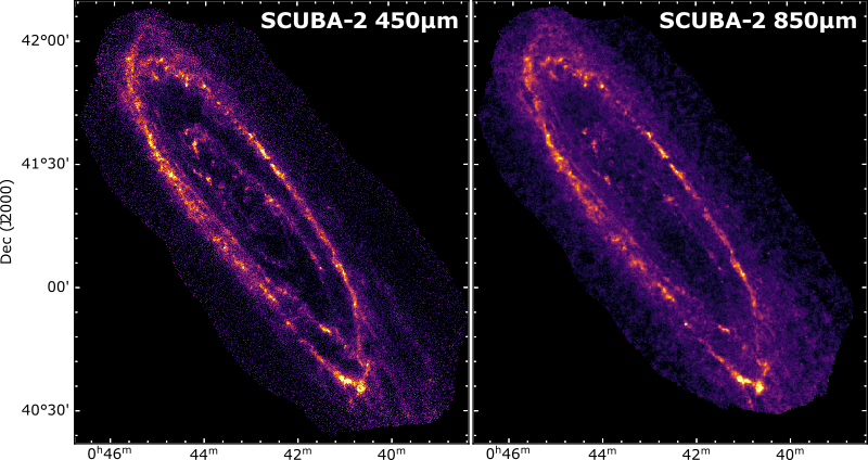
        Our SCUBA2 450 and 850 µm images from DR1. Our first SCUBA-2 Data release in September 2021 provides our SCUBA-2 maps made with ~70% of the final HASHTAG data. The maps are made with our optimised SCUBA-2 pipeline, new adapted skyloop script, and combined with space-based data to recover all spatial scales. All the software we developed is described and provided on our software page, and the full details of data release are the properties of the map are in the data release paper.

The typical sensitivity of our maps is ~2.0 and ~3 mJy beam^-1 at 850 and 450µm, respectively, with a peak sensitivity in the central regions of 1.5 and 20.6 mJy beam^-1 at 850 and 450 µm, respectively. As M31 is (most definetly) an extended source we calibrate our maps in mJy arcsec^-2, so if for example if you wish to convert to mJy per pixel multiply the map by the area of the pixel in arcsecond². As well as our images at native resolution, we also provide images that have been smoothed with Gaussian so users can bace signal-to-noise versus resolution.

The broad-band 850 µm filter includes the wavelengths where the CO(J=3-2) line is present. In our data release paper we use our CO(J=3-2) observations to predict the contamination acorss the whole disk. In general we predict the contamination to be small (mainly as M31 does not emit much CO emission) with our analysis predicting that in 80% of pixels the CO line flux is less than 0.5 K km s^-1, which corresponds to ~0.3 mJy beam^-1 (much less that our sensitivity), however, our maximum contamination predicted is 28%. Full details of our method are given in the data release paper, and our predicted CO(J=3-2) intensity map is available below.

Our SCUBA-2 maps are all multi-dimensional fits files, containing the following extensions:

0. IMAGE: The flux-density map (i.e., the normal signal map)
1. ERROR: The 'error' map showing the '1 σ' uncertainty on the flux-density measurements. This is our modified uncertainty map based on the uncertainty map produced by the pipeline and an additional contibution based on the brightness of the emission found from our simulations (see data release paper). For most use cases this is the recommended uncertainty map.
2. SENSITIVITY: The 'sensitivity' map showing the uncertainty of the flux-density measurements generated by the pipeline.

DR1 SCUBA-2 Files

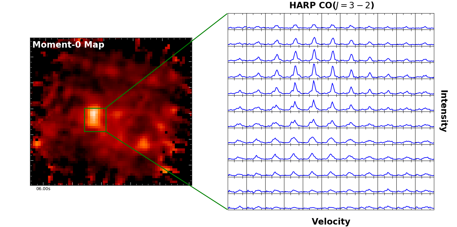
        An illustration of an of our raster CO(J=3-2) cube. For HASHTAG we target 12 regions across Andromeda with HARP on the JCMT. HARP is a 16 pixel (4×4 grid) hetrodyne instrument with an instaneous 2 GHz bandwidth (in practice for our observations typically 14 pixels were operational). In total we observe 60 square arcminutes, reaching a sensitvity of ~13 mK (T_a^*) in 1 2.6 km s^-1 channel. All details of our observations and reduction are given in Li et al. (2019)

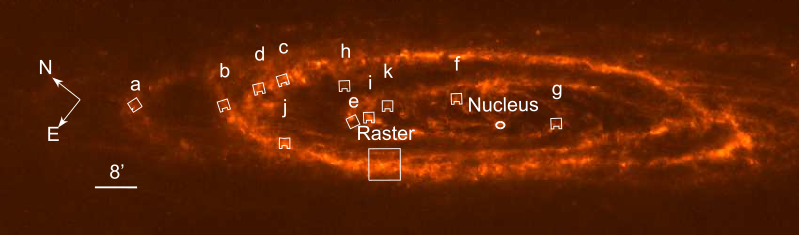
We provide two sets of cubes, one at the raw resolution of HARP and one smoothed to the same resolution as the IRAM CO(J=1-0) data. For each sets of cubes, we create a moment-0 map using the  Hi VLA data as a prior (see Smith et al. 2021) to extract the CO line. This enables us to detect the faintest lines. Moment-0 maps where channels are identified just from the cube itself are also provided which were presented in Li et al. (2019). We also provide an uncertainy map for the moment maps created with the  Hi prior. The image at below the table shows the locations of each of the fields.

CO Data Files

Data Release 1 is Now Avilable!

• Access Here!

If you from one of the EAO partners and want to get involved, go to the team page, and find your local contact. If you have any other questions about HASHTAG you can use the contact details below, or if you hvae a specific question about a paper contact the lead author.

• Matthew.Smith (at astro.cf.ac.uk)
• +44 (0)29 208 75106
• School of Physics and Astronomy
  Cardiff University, The Parade
  CF24 3AA, United Kingdom.

The JCMT is operated by the East Asian Observatory association. For more information about the JCMT and EAO click on the icon below.